Which is the Best RAID level for Video Editing and Post Production?

There are three ways to make a decision on the best RAID level for your video editing and post production needs:

• Gut feeling or instinct – also called an impulse buy.
• Years of first-hand experience running various RAID levels and systems.
• Analyzing available data to find the best odds for each RAID level.

The first-time RAID buyer should attempt to understand the complexity that goes into selecting the ‘right’ option. Too often something that looks good today will prove totally inadequate tomorrow. Those who cannot fathom or don’t want to deal with the complexity will rely on opinions or their gut feeling (If you read too many third-party opinions you’ll be more confused than ever!). You could get lucky or unlucky. The sad part is you don’t have a say in the matter either way.

If you have years of first-hand experience you wouldn’t be looking for an answer anyway. You’re already convinced about what’s best for you. This article explores the last option. Who’s it for?

I will focus on the small business post facility or single video editor. If you want to know the real-world numbers behind each RAID configuration, and are not afraid to get a bit technical to arrive at the best solution for your needs, then you will enjoy reading this article. You will ultimately do as your personality and situation dictates. I couldn’t find a similar resource to the one I’m about to show you, so I put it together.

Which RAID levels should we look at?

The RAID levels that I’ll be looking at are 0, 1, 5, 6 and 10.

These are not the only available RAID levels. There are nested RAID levels (50, 100, etc.) and proprietary/non-standard RAID levels (Z, Diff-RAID, etc.) that I won’t look at. The choices are complex as it is. The smart thing to do is begin with the easy ones.

If the RAID levels we’re covering here are inadequate for your unique needs, then you should look further.

The biggest benefit that RAID brings to the table is ‘Redundancy’ – in short, it is the ability of the system to let you continue working without delays even if there’s one or more drive failures.

The first question to ask yourself, then, is: Do you need redundancy at all? Imagine this situation:

You are editing on one 4 TB 7,200 rpm drive that sits in your computer or laptop. You have a backup on an external drive somewhere. Suddenly, your 4 TB drive fails or is erased or whatever. Here are the sequence of events that must take place to get you back to ‘as you were’:

• Format your drive (4 TB drives can take many hours, even a whole day). If it’s dead, you will replace it (Order and delivery means it’ll take days).
• Connect your external backup to your computer via USB 2.0, 3.0, eSATA or Thunderbolt (Fifteen minutes, if the drive is nearby. Maybe a day or more if the drive is in another location).
• Copy your footage to the formatted or new drive. To copy it via USB 2.0, it’ll take about 6 hours per terabyte. Via USB 3.0, Thunderbolt or eSATA, it’ll take about 3 hours per terabyte.
• Restart your NLE and hope everything links automatically (Ten minutes if everything goes well).

If your total data size is low, you might experience the loss of half a day. If your data size is significant, you will lose at least two days. If your drive dies, you might lose a week.

Of course, the smarter way to work is by having two 4TB internal drives. This way, if one crashes or dies, you can link to the other one and continue working (assuming you were alert enough to duplicate your data beforehand). The downtime in this case is about an hour not more. However, not everybody has space for two internal drives.

Can you afford to take this loss in productivity? Run the numbers based on your own data needs. If you are okay with the down time, then you don’t need RAID for redundancy.

Then, the only reason you might want RAID is speed. We’ll get to that.

The ideal drive size for a small business post facility or editor

Let’s assume you have determined that redundancy or speed is essential to your editing needs. There are many variables that go into estimating the right RAID requirements. But, there are three factors you’ll need to know right at the beginning:

• What is the total size of your data?
• What is the data rate you’ll be needing on a regular basis?
• How many layers do you typically have on your timeline overlapping each other?

The first determines the total capacity of your RAID array. The market forces you to choose the size of one drive. From the two numbers, you will arrive at the total number of drives needed to make up your required capacity. This, and the second and third factors will tell you how fast it has to be.

Working backwards to find your budget

Among all the available RAID levels that give you the capacity and speed you need, find both the cheapest and the most expensive. Does your budget lie somewhere in between?

In either case, you are limited to drive sizes that cap at 4 TB. If speed is critical, you will want to invest in 7,200 rpm drives (though 5,400 rpm or similar drives should work okay too). The cost of a 4 TB 7,200 rpm is about $300 or more (or whatever the price is). More drives means a linear increase in the total price. There’s no way of getting around it (unless you are buying hundreds of drives).

You are also limited by the connectivity options, so you cannot go about multiplying your speed. E.g., what’s the point in designing an 8-bay RAID 0 array filled with SSDs that can read at 500 MB/s. The read speed you’ll get from such a beast is about 30 Gbps. There isn’t any cheap external connectivity option that delivers data at this rate. The closest I can think of is 32G Fiber Channel.

See? You can’t aim high, and you can’t live with the low. It’s like walking into a large cave filled with treasure. There’s only so much you can carry in one trip. Finding the right RAID solution is a balancing act.

Every RAID solution offers speed. The more drives you add, the faster your array becomes. Many people automatically assume they need RAID 0 if speed is their goal. That’s rubbish. As I’ve mentioned above, you cannot multiply drives for speed without limits (just like speed limits on our roads). That means, there are options where you can have your redundancy as well as your speed – all under budget.

Which speed is the most important – write or read?

Footage recorded on set is sacrosanct. You would almost never write over it. You will only read from it.

While editing, you might render out certain scenes with effects. Or, you might create motion graphics or 3D elements that are baked in as your edit proceeds. This means, there is some writing that happens. One cannot categorically say that you’ll never write to your array. You might.

Let’s see how this affects speed. There are three major data rate ‘ranges’ in video today:

• 50 Mbps (DSLRs, Canon C300, etc.)
• 220 Mbps (Prores HQ, DNxHD 220)
• 150 MB/s (R3D, Cinema DNG from the BMCC, etc.)

Here’s the data rate (in MB/s) for the number of streams you need to read at one go:

	3	5	10
50 Mbps	18.75	31.25	62.5
220 Mbps	82.5	137.5	275
150 MB/s	450	750	1500

As you can see, at 50 Mbps, you can easily read 10 streams of 1080p content even with one 7,200 rpm drive (they deliver 100 MB/s or better). However, reading even one stream of R3D footage in full quality is tough if not impossible.

Writing offers the same problems. Leaving aside the time it’ll take your CPU or GPU to compute the new pixels, writing to the same format will essentially mean you need the same speeds, maybe more. Why more? If you’re writing to the same array being used to read the source material, your speeds will be effectively cut down by a minimum of half. E.g., if your editing timeline has four streams of footage, and you’re reading from them and rendering the composited version at the same time, your array will need enough bandwidth to manage 5 (4 read + 1 write) streams of data. That means, whatever your desired write speed is, multiply it by 5! If it’s one stream per read and one stream per write, multiply it by 2.

You see, because you are always reading from your RAID array, your RAID array will have to work extra hard to also write at the same time. For this simple reason, I strongly advise against writing to a RAID array while you’re working. The best way to manage this is to perform your renders at the end of the day or a break and come back when it’s done. If this isn’t workable, get two arrays.

Reading is the primary activity of a RAID array containing source material for editing. Reading is more important, and therefore must take absolute priority. If anything interferes with this (even if that’s writing) then that’s a bad thing.

Secondly, you might read multiple streams at the same time (that’s the nature of editing), but you’ll hardly ever write more than one stream at the same time. Most batch rendering applications perform one render at a time. You can safely say that no matter what you do, it’ll be safe to design a RAID array in this way:

• Desired read speed = Number of read streams x data rate. It would be very rare for the number of streams to exceed 5.
• Desired write speed = data rate of rendered format.

What does that tell you? The read speed is at least twice as important as the write speed. On average, it is three times more important.

Read and Write speeds of various RAID levels

Let’s look at the theoretical read and write speeds offered by various RAID levels.

Notes: I’m assuming the following:

• Drive speed (read or write) is 100 MB/s, though you have faster platter drives.
• Drive size is 4 TB.
• Price of a 4 TB drive is $300.
• Failure rate of a 4 TB drive is 5% (You buy a 100 and five will fail within the first year).

On the left is the number of drives in the array. Speeds are in MB/s.

Read speeds

	Read Speed (MB/s)
Drives	0	1	5	6	10
2	200	200	x	x	x
3	300	300	200	x	x
4	400	400	300	200	400
5	500	500	400	300	x
6	600	600	500	400	600
7	700	700	600	500	x
8	800	800	700	600	800
9	900	900	800	700	x
10	1000	1000	900	800	1000
11	1100	1100	1000	900	x
12	1200	1200	1100	1000	1200
13	1300	1300	1200	1100	x
14	1400	1400	1300	1200	1400
15	1500	1500	1400	1300	x
16	1600	1600	1500	1400	1600
32	3200	3200	3100	3000	3200
64	6400	6400	6300	6200	6400

x – RAID 5 needs a minimum of 3 drives. RAID 6 and 10 needs a minimum of 4 drives. RAID 10 needs an even number of drives.

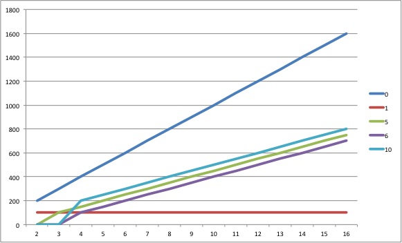
If looking at the table is giving you headaches, here’s a simple graph of the same table:

It doesn’t take a rocket scientist to realize that all RAID levels offer a linear increase in read speed as you increase the number of drives. RAID 10 and RAID 1 are as fast as RAID 0. RAID 5 and 6 are no slouches either.

See? Speed does not categorically mean RAID 0. Get that out of your head.

Write speeds

Write speeds are a bit weirder. From this point on we enter the twilight zone. Brace yourselves.

Most drives offer a slightly lower write speed when compared to read speeds. It’s not because of any physical thing but simply because the drive needs to find the right spot to write data in before it can write. This additional calculation makes it slower than reading. For simplicity’s sake, I’m going to assume that the write speed is equal to the read speed. When you make calculations in the real world, you’ll never be at the limit. You must always account for some wastage or loss. I’m assuming your total data rate is well below both the read and write limits of your drive.

So, if we assume the write speed is the same as the read speed, then, in an ideal world, the write graph should look like this:

However, this doesn’t happen in practice. For RAID 5 and 6, data isn’t duplicated. Instead, parity data is calculated and written alongside the actual write data. E.g., if your write data rate is 100 MB/s, in reality a RAID 5 or RAID 6 array will write 100+x MB/s (x is parity). It gets even more complicated. If you are overwriting data (rendering a new version of a composition or chroma key, for example) then the old parity data needs to be read, and only then will the new one be calculated. Then, the new one will be compared to the old one to see if it needs to be changed, and then the writing takes place.

RAID 5 and 6 perform worse for sequential data (video is sequential data) because that many more calculations have to happen per second.

There are various factors that affect the overall speed of writing parity data. The most important is the RAID Controller that must calculate the parity data before writing it. The really good (expensive) controllers have correct caching to eliminate a lot of this time wastage. The cheaper hardware RAID controllers don’t do this so well. For this reason, there is no universal formula for calculating the average write speeds for RAID 5 and RAID 6 arrays, but they’ll look something like this in the best case:

Drives	Write Speed (MB/s)
	0	1	5	6	10
2	200	100	x	x	x
3	300	100	100	x	x
4	400	100	150	100	200
5	500	100	200	150	x
6	600	100	250	200	300
7	700	100	300	250	x
8	800	100	350	300	400
9	900	100	400	350	x
10	1000	100	450	400	500
11	1100	100	500	450	x
12	1200	100	550	500	600
13	1300	100	600	550	x
14	1400	100	650	600	700
15	1500	100	700	650	x
16	1600	100	750	700	800
32	3200	100	1550	1500	1600
64	6400	100	3150	3100	3200

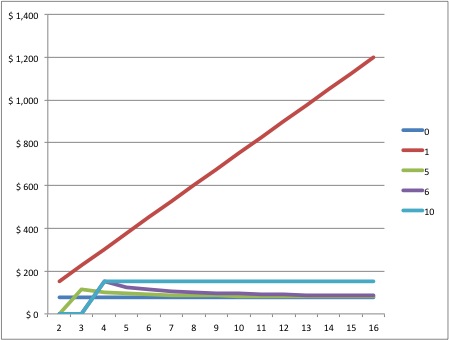
And here’s the graph:

RAID 1 is good with two drives. Adding drives to a RAID 1 does not increase write speed in any way. RAID 0 is best, and every other RAID is similar (Don’t forget, RAID 5 and 6 only perform this way with really good hardware RAID Controllers, otherwise the performance is going to be very poor). As a rule of thumb, you can estimate the write speeds for a RAID 5 or 6 array to be 25% or lower than the read speed. I’ve estimated it at 50% because that’s the best that you can get.

Which RAID level gives the best capacity?

Here are the various RAID levels compared on actual capacity according to the number of drives (size of one drive is 4 TB):

Drives	Total Capacity (TB)
	0	1	5	6	10
2	8	4	x	x	x
3	12	4	8	x	x
4	16	4	12	8	8
5	20	4	16	12	x
6	24	4	20	16	12
7	28	4	24	20	x
8	32	4	28	24	16
9	36	4	32	28	x
10	40	4	36	32	20
11	44	4	40	36	x
12	48	4	44	40	24
13	52	4	48	44	x
14	56	4	52	48	28
15	60	4	56	52	x
16	64	4	60	56	32
32	128	4	124	120	64
64	256	4	252	248	128

And here’s the graph:

RAID 1 is the biggest loser here. Once you cross two drives, you are just duplicating the same data to every additional drive. The total capacity of a RAID 1 drive is always equal to the capacity of one drive.

RAID 10 has a 50% drive penalty, because in affect it behaves like a RAID 1, had it been capable of scaling up. RAID 5 and RAID 6 do much better, because they don’t have to duplicate data, but just write a few parity bits which don’t require a lot of overhead.

RAID 0 is the best, because it gives you the full capacity of each drive. Don’t forget to note that if a drive is rated at X TB, the actual capacity is always a bit smaller.

If you’re short on cash and absolutely need to make the most out of every drive, the above chart tells you which options to go for. This is why RAID 5 is very popular. It gives you a lot of space, and offers you some protection (redundancy). But it comes at a price, which we’ll see soon.

Which RAID level is the cheapest on a Cost per terabyte basis?

Obviously, if an array cannot use up all its capacity, then the cost per terabyte goes up. Let’s see by how much:

Drives	Cost/TB
	0	1	5	6	10
2	$ 75	$ 150	x	x	x
3	$ 75	$ 225	$ 113	x	x
4	$ 75	$ 300	$ 100	$ 150	$ 150
5	$ 75	$ 375	$ 94	$ 125	x
6	$ 75	$ 450	$ 90	$ 113	$ 150
7	$ 75	$ 525	$ 88	$ 105	x
8	$ 75	$ 600	$ 86	$ 100	$ 150
9	$ 75	$ 675	$ 84	$ 96	x
10	$ 75	$ 750	$ 83	$ 94	$ 150
11	$ 75	$ 825	$ 83	$ 92	x
12	$ 75	$ 900	$ 82	$ 90	$ 150
13	$ 75	$ 975	$ 81	$ 89	x
14	$ 75	$ 1,050	$ 81	$ 88	$ 150
15	$ 75	$ 1,125	$ 80	$ 87	x
16	$ 75	$ 1,200	$ 80	$ 86	$ 150
32	$ 75	$ 2,400	$ 77	$ 80	$ 150
64	$ 75	$ 4,800	$ 76	$ 77	$ 150

And here’s the graph:

It is instructive to know that RAID 0 and RAID 10 have no impact on the cost per TB, no matter how many drives you buy. This means scaling up has no benefits unless the drive vendor gives you any discounts.

On the other hand, RAID 5 and RAID 6 gets cheaper as you increase the number of drives, regardless of any discounts you get for the actual drives.  They do stagnate after a point, though – which is about the 32-drive mark. Interestingly, once you increase the number of drives to 64 or more, RAID 6 actually catches up with RAID 5 in terms of cost per TB; and they both catch up with RAID 0. But 64 is a large number of drives for one array, and you’ll be lucky to find a controller (or stacking controllers even) with that many connectors!

RAID 1, though, is a total waste of money beyond two drives, but we knew that already.

Drive and Array failure rates for various RAID levels

There are two things to consider when looking at the failure rate of a RAID array:

• How many drives can fail?
• What are the chances of failure?

The number of drives that can fail for different RAID levels

Here’s how they stack up:

Drives	How many drives can fail
	0	1	5	6	10*
2	0	1	x	x	x
3	0	2	1	x	x
4	0	3	1	2	2
5	0	4	1	2	x
6	0	5	1	2	3
7	0	6	1	2	x
8	0	7	1	2	4
9	0	8	1	2	x
10	0	9	1	2	5
11	0	10	1	2	x
12	0	11	1	2	6
13	0	12	1	2	x
14	0	13	1	2	7
15	0	14	1	2	x
16	0	15	1	2	8
32	0	31	1	2	16
64	0	63	1	2	32

*Half the number of drives in a RAID 10 array can fail, but only one from each span. E.g., if you divide your 16-bay array into 8 groups, then only one drive per group can fail (or 8 drives total). The actual calculation of the probability of failure for RAID 10 is far more complicated.

And here’s the graph:

Obviously, RAID 0 performs poorly. No matter how many drives you add, a RAID 0 array will not tolerate a single drive failing. RAID 1 performs best, because it just duplicates data into as many drives as you can add. RAID 6 offers better protection than RAID 5, and I guesstimate that RAID 10 offers better odds than RAID 6.

The failure rate of a RAID array

How does the number of drives affect the failure rate of an entire array? Here are the stats:

Drives	Array failure rate
	0	1	5	6	10**
2	10%	0.25%	x	x	x
3	14%	0.01%	3%	x	x
4	19%	0.00%	5%	3%	0.186%
5	23%	0.00%	7%	5%	x
6	26%	0.00%	10%	7%	0.397%
7	30%	0.00%	12%	10%	x
8	34%	0.00%	14%	12%	0.673%
9	37%	0.00%	16%	14%	x
10	40%	0.00%	19%	16%	1.003%
11	43%	0.00%	21%	19%	x
12	46%	0.00%	23%	21%	1.379%
13	49%	0.00%	25%	23%	x
14	51%	0.00%	26%	25%	1.793%
15	54%	0.00%	28%	26%	x
16	56%	0.00%	30%	28%	2.239%
32	81%	0.00%	54%	52%	6.450%
64	96%	0.00%	80%	79%	15.4%

**Calculating the failure rate of a RAID 10 array isn’t easy. I’ve used a simple formula that might be totally incorrect. Each RAID 10 array is split into n/2 RAID 1 spans where n is the total number of drives. The failure rate of each span is equal to 0.25%, the failure rate of a 2-drive RAID 1 array. All these spans are striped (RAID 0), and as the number of spans increases, the chances for failure rises (just like RAID 0). The formula I’ve used for RAID 10 = rate of RAID 1 (0.25%) x number of spans (n/2) x rate of RAID 0 for n/2, which is the number of spans.

Here’s the graph:

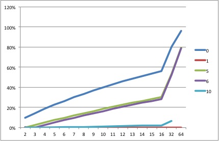
Obviously, RAID 0 is dangerous even with two drives. But as you increase drives it becomes an unacceptable risk. E.g., If you have about 12 drives in RAID 0, the chance of failure is 50:50 – that means anytime. If you have 64 drives, it’s almost a 100% – which means failure is imminent. What’s the difference? With 12 drives, you get to flip a coin. With 64 drives, you get to flip a coin, but it’s given to you by Two-Face.

RAID 1 is the simplest way to go if all you needed were two drives. Add one more to a RAID 1 array and you’ll be as safe as possible. The same applies to RAID 10 – the sheer number of drives makes failure in the real world a minimal possibility, even for smaller arrays. But it is an uncomfortable peace.

But look at RAID 5 and RAID 6. They’re both unacceptably dangerous as you increase the size of your array. Remember what I said about not being able to carry out all the treasure from the cave in one go? So far RAID 5 and RAID 6 have seemed like great solutions, but not for large drive arrays. There’s always a trade-off with RAID somewhere.

Bringing everything down to one number

What are the things we’re worried about most when building a RAID array? Here are some important points:

• Total capacity
• Value for money
• Redundancy
• Speed

There are others, too:

• Ease of setup
• Cost and availability of hardware RAID controllers
• Number of drives and size of chassis and heating solutions
• Compatibility of hardware and software
• CPU usage
• Battery Backup for the controller
• Caching
• Buying drives from various sources to better the odds

Let’s focus on the first four for now. That offers us a theoretical starting point. After all, if a RAID level doesn’t work for us theoretically, there’s no point worrying about its technicalities.

The objective is to bring each important point to a common number. Luckily, RAID offers us simple formulas that can be scaled equally among all levels. E.g., if a drive is slow or if its failure rate is high, every RAID level suffers. If the price changes, everyone’s affected equally.

Mathematically, there are an infinite number of ways in which such numbers can be produced. I’m going for the simplest method, possibly the most error-prone, but who cares as long as it makes some sense? The two types of numbers I’m going to be reducing our data to are:

• Factors
• Value

Factors

A factor mustn’t have a unit. It’s just a number that should ideally be between 0 and +1. 1 being the best and 0 being the worst.

Value

You will spend X amount of money on your RAID array. But how much value do you get out of it? Obviously this is a subjective matter because each individual perceives value differently. Just for fun, I multiply the total cost of the array by the factor I’ve obtained to get the value.

Let’s see how this works in practice.

Speed factor

We have seen that on average the ability of a RAID array to read quickly is three times more important than its ability to write fast. The ‘Speed Factor’ (S) should include both read and write speeds (you can’t buy them separately you know). I used this formula:

Speed Factor (S) = (3 x Read speed + 1 x Write Speed) / (4 x Maximum speed of the array)

Here’s what we get:

Drives	Speed factor (S)
	RAID 0	RAID 1	RAID 5	RAID 6	RAID 10
2	1.000	0.875	x	x	x
3	1.000	0.833	0.583	x	x
4	1.000	0.813	0.656	0.438	0.875
5	1.000	0.800	0.700	0.525	x
6	1.000	0.792	0.729	0.583	0.875
7	1.000	0.786	0.750	0.625	x
8	1.000	0.781	0.766	0.656	0.875
9	1.000	0.778	0.778	0.681	x
10	1.000	0.775	0.788	0.700	0.875
11	1.000	0.773	0.795	0.716	x
12	1.000	0.771	0.802	0.729	0.875
13	1.000	0.769	0.808	0.740	x
14	1.000	0.768	0.813	0.750	0.875
15	1.000	0.767	0.817	0.758	x
16	1.000	0.766	0.820	0.766	0.875
32	1.000	0.758	0.848	0.820	0.875
64	1.000	0.754	0.861	0.848	0.875

And here’s the graph:

For simplicity’s sake, I’m not showing you the value chart but you can multiply the cost of the array with the speed factor to get the Value for Speed (ValueS) for each array. Here’s what it looks like on a graph:

If all you cared for was speed, it is pretty obvious that RAID 0 is the way to go, followed quickly by RAID 10. As far as value for money for speed is concerned, RAID 0 is ideal, followed by RAID 10.

Capacity factor

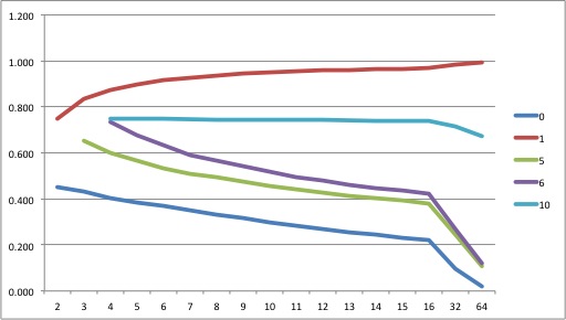
The capacity factor is easier to calculate. It is:

Capacity Factor (C) = Actual capacity of the array / Maximum possible capacity

Here is the chart:

Drives	Capacity Factor (C)
	RAID 0	RAID 1	RAID 5	RAID 6	RAID 10
2	1.000	0.500	x	x	x
3	1.000	0.333	0.667	x	x
4	1.000	0.250	0.750	0.500	0.500
5	1.000	0.200	0.800	0.600	x
6	1.000	0.167	0.833	0.667	0.500
7	1.000	0.143	0.857	0.714	x
8	1.000	0.125	0.875	0.750	0.500
9	1.000	0.111	0.889	0.778	x
10	1.000	0.100	0.900	0.800	0.500
11	1.000	0.091	0.909	0.818	x
12	1.000	0.083	0.917	0.833	0.500
13	1.000	0.077	0.923	0.846	x
14	1.000	0.071	0.929	0.857	0.500
15	1.000	0.067	0.933	0.867	x
16	1.000	0.063	0.938	0.875	0.500
32	1.000	0.031	0.969	0.938	0.500
64	1.000	0.016	0.984	0.969	0.500

And here is the graph:

The value for money for capacity (ValueC) is as follows:

RAID 0 is the best if capacity is your only concern. However, RAID 5 and RAID 6 both offer excellent value as the number of drives go up. RAID 10 offers half the value.

Failure factor

The failure factor is complicated, and is possibly the most error-prone part of my calculations. Array failure rates depend on the failure rate of a drive (constant) and the number of drives. However, each RAID type also differs in the number of drives that can fail. I feel both these variables must be accounted for in the Failure Factor (F).

The first step is to find the drive failure factor, which is the number of drives that are allowed to fail divided by the total number of drives. Let’s call this ‘d’. To keep things simple I’m not showing you that chart. You should know that I changed the RAID 0 value (0) to 0.001 just so we don’t encounter a ‘divided by zero’ scenario. We have already calculated the array failure rate earlier.

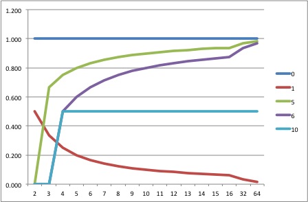
Resistance to Failure Factor (F) = (1-Array Failure Rate+d) / 2

I wanted to create the factor such that the higher number offered greater ‘protection’. This makes all factors behave commonly – the higher the better. All I’ve done is average the two, by giving both factors equal importance.

Here’s the chart:

Drives	Resistance to Failure Factor (F)
	RAID 0	RAID 1	RAID 5	RAID 6	RAID 10
2	0.450	0.749	x	x	x
3	0.430	0.833	0.652	x	x
4	0.405	0.875	0.600	0.735	0.749
5	0.385	0.900	0.565	0.675	x
6	0.370	0.917	0.533	0.632	0.748
7	0.350	0.929	0.511	0.593	x
8	0.330	0.937	0.493	0.565	0.747
9	0.315	0.944	0.476	0.541	x
10	0.300	0.950	0.455	0.520	0.745
11	0.285	0.955	0.440	0.496	x
12	0.270	0.958	0.427	0.478	0.743
13	0.255	0.962	0.413	0.462	x
14	0.245	0.964	0.406	0.446	0.741
15	0.230	0.967	0.393	0.437	x
16	0.220	0.969	0.381	0.423	0.739
32	0.095	0.984	0.246	0.271	0.718
64	0.020	0.992	0.108	0.121	0.673

Here’s the graph:

And here’s the value for money for resistance (ValueF) graph:

RAID 1, in pure protection terms, is always the best, regardless of the number of drives. RAID 10 is the next best thing. RAID 0 is the worst.

Results

The R Factor

The idea behind creating three factors is to multiply them to form one final factor – R.

R = S x C x F

This offers some flexibility, though. What if you didn’t care about capacity, for example? In that case, ignore it, and R = S x F. You can ignore two factors and just focus on one thing. Choose any combination you want.

I’m going to leave the permutations and combinations to you, and will only provide the results of combining all three factors. Here’s the chart:

Drives	R Factor
	0	1	5	6	10
2	0.450	0.328	x	x	x
3	0.430	0.231	0.253	x	x
4	0.405	0.178	0.295	0.161	0.328
5	0.385	0.144	0.316	0.213	x
6	0.370	0.121	0.324	0.246	0.327
7	0.350	0.104	0.329	0.265	x
8	0.330	0.092	0.330	0.278	0.327
9	0.315	0.082	0.329	0.286	x
10	0.300	0.074	0.322	0.291	0.326
11	0.285	0.067	0.319	0.290	x
12	0.270	0.062	0.314	0.291	0.325
13	0.255	0.057	0.308	0.289	x
14	0.245	0.053	0.306	0.287	0.324
15	0.230	0.049	0.300	0.287	x
16	0.220	0.046	0.293	0.283	0.323
32	0.095	0.023	0.202	0.209	0.314
64	0.020	0.012	0.091	0.099	0.295

And here’s the graph:

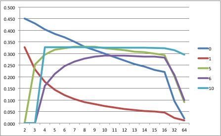
What does this tell us? In no uncertain terms:

• If your RAID array is between 2-8 drives large, RAID 0 is best.
• If your RAID array is between 8-10 drives large, RAID 5 is best.
• If your RAID array is greater than 10 drives, RAID 10 is best.

What?? How can RAID 0 be best, even though we all know a single drive failure will ruin our work? We have already calculated the array failure rate for each RAID array. To find how many years the array will survive based on those rates, look at this table:

Drives	Life Expectancy (years)
	0	1	5	6	10
2	10	400	x	x	x
3	7	–	33	x	x
4	5	–	20	33	526
5	4	–	14	20	x
6	4	–	10	14	256
7	3	–	8	10	x
8	3	–	7	8	147
9	3	–	6	7	x
10	3	–	5	6	100
11	2	–	5	5	x
12	2	–	4	5	72
13	2	–	4	4	x
14	2	–	4	4	56
15	2	–	4	4	x
16	2	–	3	4	45
32	1	–	2	2	15
64	1	–	1	1	7

What is the typical warranty period of a hard drive? Three years? So, one can safely say that a RAID array must ‘live’ for three years before it fails (which it will – all arrays will fail at some point). Going by that, a RAID 0 array with 10 drives will live for three years.

A RAID 5 or 6 array with 16 drives will live up to three years; and a RAID 10 drive with 64+ drives will live longer than 3 years. RAID 1 of course, lives up to 400 years even with two drives. Remember, RAID is NOT backup. Regardless of what RAID you choose, you must always keep backups of your data. When you know you have sufficient backups, an array failure is no longer such a fearful thing, is it?

And don’t forget, your RAID array can be brought to its knees by the controller, the motherboard, the CPU, RAM, the OS, or just human error.

On the one hand we are bombarded with information on how dangerous RAID 0 is, but the numbers don’t support that FUD. But what about bad luck, you might be wondering. Bad luck can happen to anybody at any time. There is no mathematical basis for luck, only chance. You either believe in luck (didn’t I tell you you could select a RAID array with just your gut feeling?) or believe in chance. It’s not for me to decide for you.

Go make your own luck.

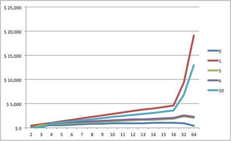
Value for money

What about value for money? Here’s the formula:

Value for Money (V) = (ValueS + ValueC + ValueF ) / 3

Here’s the chart:

Drives	Value for money (V)
	RAID 0	RAID 1	RAID 5	RAID 6	RAID 10
2	$ 490	$ 425	x	x	x
3	$ 729	$ 600	$ 571	x	x
4	$ 962	$ 775	$ 803	$ 669	$ 850
5	$ 1,193	$ 950	$ 1,033	$ 900	x
6	$ 1,422	$ 1,125	$ 1,258	$ 1,129	$ 1,274
7	$ 1,645	$ 1,300	$ 1,483	$ 1,353	x
8	$ 1,864	$ 1,475	$ 1,707	$ 1,577	$ 1,697
9	$ 2,084	$ 1,650	$ 1,928	$ 1,800	x
10	$ 2,300	$ 1,825	$ 2,143	$ 2,020	$ 2,120
11	$ 2,514	$ 2,000	$ 2,360	$ 2,233	x
12	$ 2,724	$ 2,175	$ 2,575	$ 2,449	$ 2,542
13	$ 2,932	$ 2,350	$ 2,788	$ 2,663	x
14	$ 3,143	$ 2,525	$ 3,006	$ 2,875	$ 2,963
15	$ 3,345	$ 2,700	$ 3,215	$ 3,093	x
16	$ 3,552	$ 2,875	$ 3,423	$ 3,301	$ 3,382
32	$ 6,704	$ 5,675	$ 6,599	$ 6,493	$ 6,696
64	$ 12,928	$ 11,275	$ 12,503	$ 12,397	$ 13,108

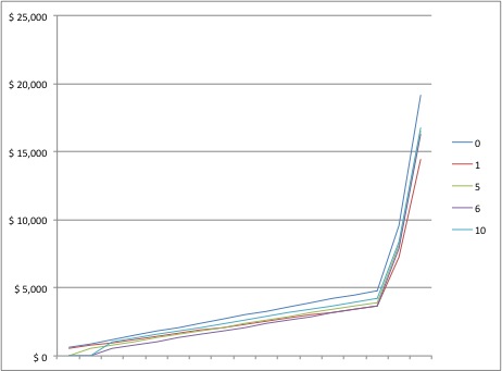
Here’s the graph:

Only RAID 1 falls behind as the number of drives increases, but generally, all RAID levels are good value for money! RAID 0 being the best until a drive count of 64, where RAID 10 takes over.

Takeaways

The numbers, as far as I can tell, don’t lie:

• For 2-8 drives, you’ll be safe with RAID 0.
• For 8-10 drives, you’ll be happy with RAID 5.
• For more than 10 drives, you’ll be thrilled to have RAID 10.

What should you pick? It’s not always this difficult. The total size of your array, your data rate and budget will limit your possibilities. Within that, you can use my methodology to come to a final decision. You could either give all factors equal importance, or leave out the ones you don’t care about.

You could assume that you will not accept anything less than five years life-expectancy for your drive array. In that case RAID 0 works great for up to 4 drives, and RAID 10 beyond that point. Heck, even if you chose each factor one at a time, it is difficult to argue against RAID 0 or RAID 10.

Going by our charts, RAID 5 and RAID 6 doesn’t look good for the kind of work we are into at all! That’s actually a relief, because you really don’t need to spend extra on RAID controllers when you can use software RAID. Look at the operating systems that support RAID 0, 1 and 10:

• Windows 8**
• Linux+mdadm
• Mac OS X

**Windows 8 has a feature called Storage Spaces that let you create something similar to RAIDs 0, 1 and 5, but not RAID 10. However, Windows also has a software RAID option for striping (RAID 0). You can combine the two to create a RAID-10-like array.

Let’s consider some of the other factors we listed earlier:

• Ease of setup – RAIDs 0 and 1 are the easiest to set up, followed by RAID 10.
• Cost and availability of hardware RAID controllers – the problem with RAID controllers is that if it fails, you will have to find a ‘matching’ model that supports your existing array.
• Number of drives and size of chassis and heating solutions – RAID 0 will keep your drives to a minimum. RAID 10 takes the most drives.
• Compatibility of hardware and software – See above.
• CPU usage – If no parity calculations are required, you don’t need to tax your CPU.
• Battery Backup for the controller – No controller means no Battery Backup Module (BBM) required. Here, too, compatibility is a problem.
• Caching – Hardware caching is always a good thing.
• Buying drives from various sources to better the odds – is common to all RAID arrays, accept maybe RAID 1.

You do the math.

But spell it out dammit! Which is the best RAID level for video?

I’m not mincing words: RAID 0 is the best RAID level for video up to 8 drives. After that point RAID 10 is champion.